Td5 Tuning

EU3 Specific Limiters

Friday, September 13, 2019 - 08:45

The 3.0 release of the XDFs includes two additional EU3 specific limiters. Both limiters use ambient air temperature (AAT) as part of the calculation of the parameter value. This makes them slightly problematic as Nanocom omits this value from display and logs despite reading the data from the ECU. Fortunately the calculations don’t seem overly sensitive to AAT so an estimation will likely suffice.
If you are estimating its worth understanding what AAT is...

AAT is not Ambient

While it’s been claimed in various places that the AAT sensor measures “ambient temperature” this somewhat misleading. The AAT sensor is measuring air temperature inside the lid of the airbox and can be significantly higher than external ambient temperature.
The airbox temperature is effectively "pre-heated" by under bonnet temperatures, so engine, radiator, turbo, and even sun on the bonnet have an impact.

AAT and ECT

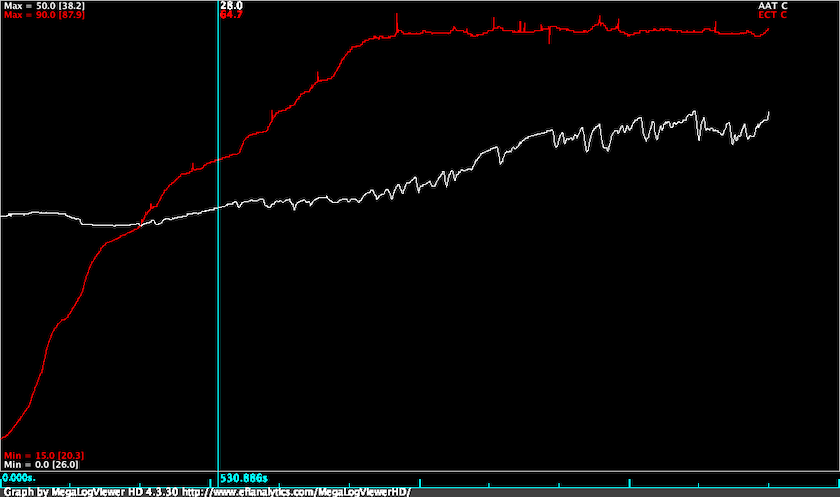
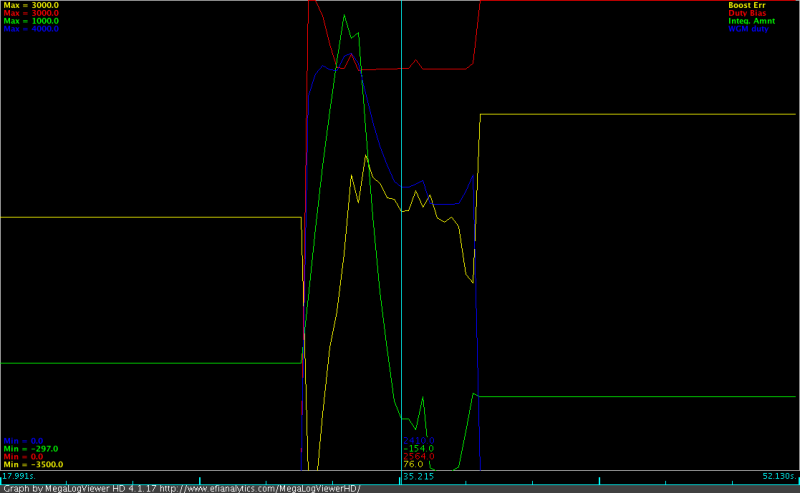
You can see from the logged data above that from a cold start AAT is reading around 26°C. As the engine and coolant warms up under bonnet temperatures increase and “ambient” temperature rises. AAT peaks at 38°C when the vehicle is idling at the end of the log. So in this example there is a 12 degree differential between AAT when the engine is cold and when the engine is hot and idling.

MAF, AAT and ECT

The other factor to consider is that increased air flow reduces the AAT reading.
As can been seen in the zoomed section of the plot, there was a 2.8 degree drop in AAT when there is high flow through the airbox compared with the no load flow.

The take away is if you need to guesstimate assume AAT will be higher than ambient temperature by something like 10°C.

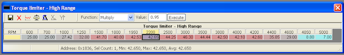
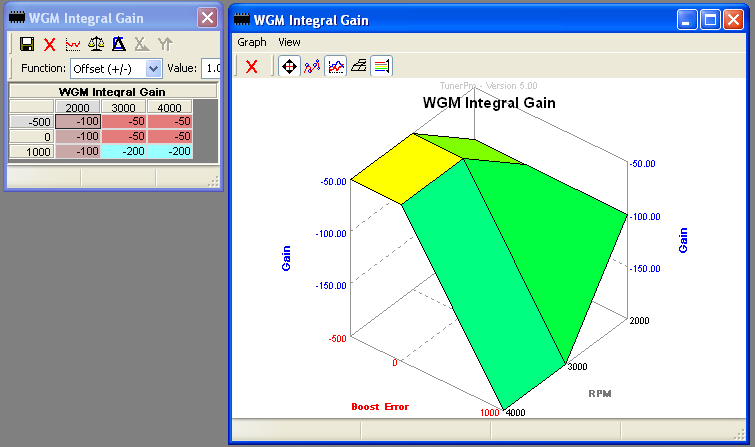
Over temp multiplier

This table is apparently used to limit fuelling to protect against excessive exhaust gas temperatures.

If you look at the table values you’ll see that the limiter has no influence below 3000rpm, nor when the Y axis parameter is at or below the minimum value.

The Y axis parameter is calculated from ambient pressure and temperature:
$$param = \frac{(AAT + 273.2) \cdot 50}{300} + \frac{25 \cdot 100}{AAP}$$

where AAT is °C and AAP is kPa.

If you were at 2000m where standard pressure is 81kPa, and you had an AAT reading at 35°C the limiter parameter would be: $$param = \frac{(35 + 273.2) \cdot 50}{300} + \frac{25 \cdot 100}{81}$$
$$param = 82 = 0.82$$

This value is high enough to trigger limiting above 3500rpm.

The parameter calculation is roughly twice as sensitive to decrease in AAP as it is to increase in AAT. You'd need extreme AAT values in the range of 70-80°C to cause limiting at sea level.

Where this may become a factor is on high road passes - Stelvio Pass is 2757m ASL for example. At this altitude standard pressure is around 74kPa, so you'd be seeing limiting creeping in above 300rpm with 40°C AAT.

It is likely that this limiter will only rarely need to be touched, if ever.
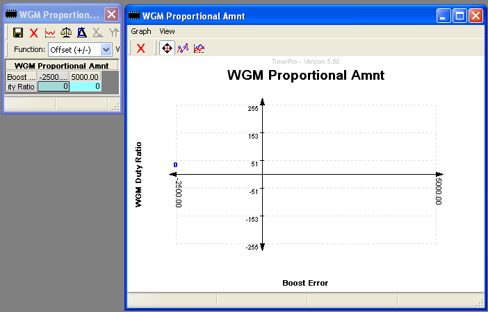
Turbo Overspeed

The Turbo Overspeed limiter is a bit of a silent killer in the EU3 maps.

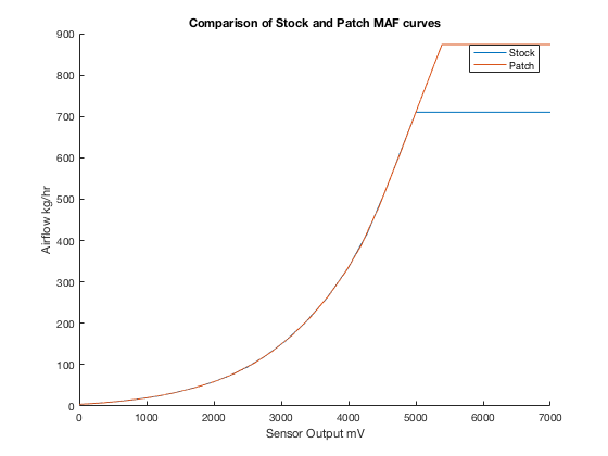
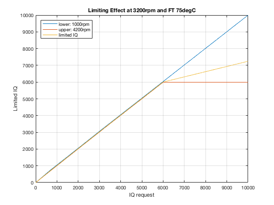
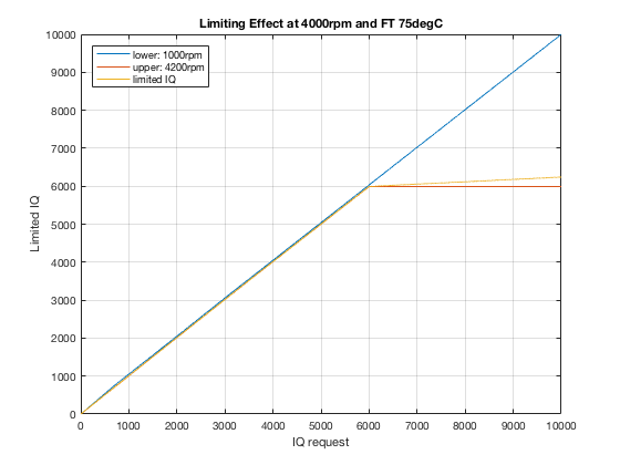
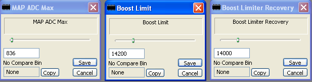
The limiter begins reducing fuel once operating conditions reach the equivalent of 1.5 bar boost and 680kghr MAF at sea level.

The exact limiting threshold will change with ambient pressure and temperature, manifold pressure, and mass air flow.

Working with the values in kPa, kg/hr and °C the main parameter calculation for the overspeed limiter is: $$ param = \frac{MAP + 0.0424 \cdot MAF \cdot \sqrt{AAT + 273.2}}{AAP}$$

The parameter calculation can be thought of having three main components:

  1. pressure ratio
  2. flow rate
  3. turbo speed constant

Pressure Ratio

This is a measure of input pressure (AAP) to output pressure (MAP). I’m ignoring the pressure drop caused by intercooler here, so:

$$pr =\frac{MAP}{AAP}$$ As an example lets look at pressure ratio required to produce 135kPa boost at AAP = 100kPa and 80kPa. $$pr = \frac{235}{100} = 2.35$$ $$pr = \frac{215}{80} = 2.69$$

You’ll see from the turbo map that turbine speed increases with pressure ratio. This means to produce the same output pressure turbine speed must increase as altitude increases.

Flow rate

The flow rate is determined as:

$$fr = \frac{MAF\times\sqrt{AAT K}}{AAP}$$

Assuming a temperature drop of 9.8°C per 1000m and 25°C ambient at sea level, and MAF = 500kg/hr.

At sea level: $$\frac{\sqrt(25+273.2)}{101} = \frac{17.27}{101} = 0.171$$ $$fr = 500 * 0.171 = 85.5$$

At 2000m ASL: $$\frac{\sqrt(5.4+273.2)}{101} = \frac{16.69}{80} = 0.209$$ $$fr = 500 * 0.209 = 104.5$$

A decrease in ambient pressure and turbo inlet temperature results in an increase in flow rate multiplier.

tb_speed_const

This is a scalar value set to 0.0424 in all fuel maps. This is incorrectly scaled in the 3.0 XDFs. The issue is fixed in 3.1 release.

Reassemble the components…

If we look at the parameter equation in terms of blocks we have this: $$param = pr + fr \times speedConst$$

So using the above values for sea level: $$param = 2.35 + 85.5 \times 0.0424 = 5.97$$ and 2000m: $$param = 2.69 + 104.5 \times 0.0424 = 7.13$$

The Overspeed limiter x-axis starts at 7.0, with no limiting applied below this parameter value.

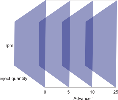
Two it would appear that his calculation uses what are effectively the x and y axes of a turbo performance map to create a limiter that accounts for the effect of air density on turbine speed.

To further illustrate I’ve mapped the 7.0 parameter value for 680kg/hr MAF at sea level onto a GT2052S 52 trim performance map.

Annotated GT2052 map
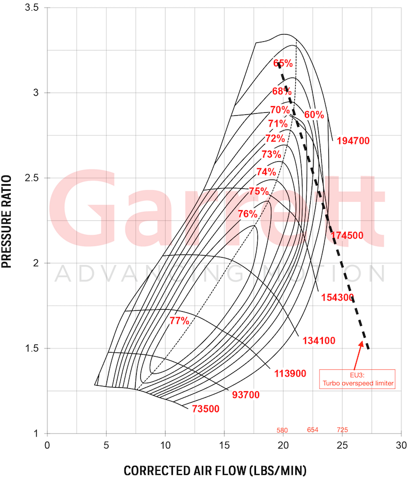
Note the figures in red above the x-axis are MAF in kg/hr.

Because this is a calculated parameter the only way to fully assess whether this limiter is actually impacting is to calculate using the above formula from log data.

This can be done with a spreadsheet app or using a calculated field in MegaLogViewerHD.

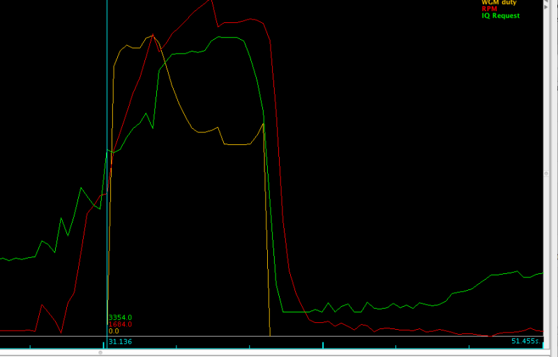
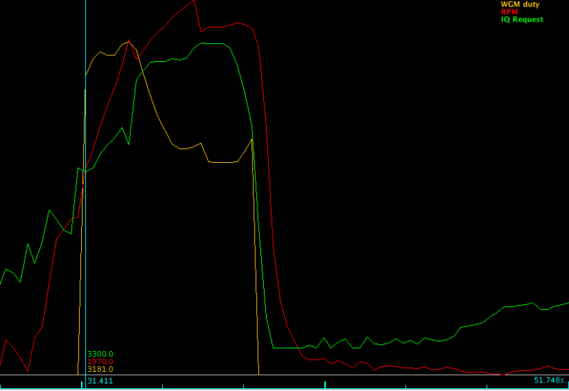
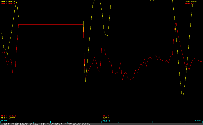
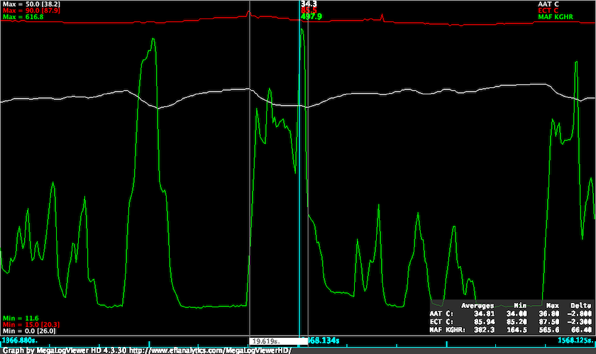
As a final illustration of the effect of this limiter, I’ll include a small segement of a log from a site donor who was having some major issues with a hybrid turbo and map levels over 250kPa.

OS Limiter in action

The white trace is request IQ after Driver Demand and Torque/Smoke limiters.
The red trace is the IQ after application of the all system limiters including the Turbo Overspeed map.

The point at the cursor shows a 26% reduction in requested IQ corresponding to the 7.5 cell in the limiter map.

You can also see clearly that as the OS limiter parameter increases above 7.0 the IQ after all limiters reduces. MAP levels when limiting is occurring are around 250-260kPa.

The take away is simple:
If you are running boost above 250 kPa on an EU3 with a "new school" map this limiter is kicking your butt.

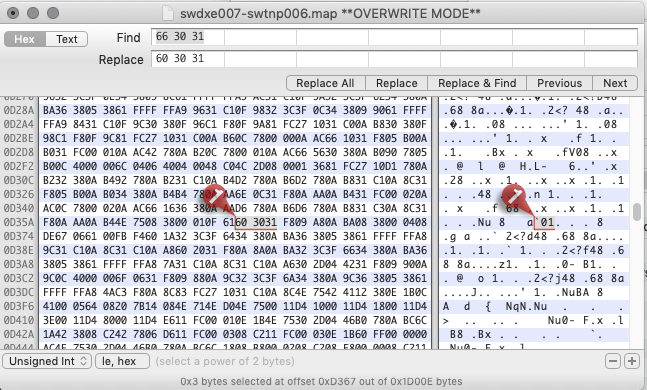
Adjusting the limiter

Rather than modifying the limiter table I would suggest altering the tb_speed_const.

  1. Work out max Pressure Ratio at sea level - this MAP divided by AAP $$275kPa / 100kPa = 2.75$$

  2. Subtract that from 7.0 to get your flow component. $$fc = 7.0 - 4.25$$

  3. Work out your maximum MAF multiply and multiply by 0.1738 to get flow rate $$720 \times 0.1738 = 125$$

  4. Divide the flow component by flow rate to find tb_speed_const: $$4.25 / 125 = 0.034$$

A note GT2052S turbo maps

The Garrett catalog and website list three different compressor trims for the stock GT2052S turbo: 48, 50 and 52. There are two maps available for the 52 trim version. The newest of these, which shows an extended range to a pressure ratio of 3.5, is on Garrett website. The others can be found in Garrett catalogs.

The problem here is that the Td5 uses the 54 trim compressor, and there is no publically avaliable map. The 52 trim will be the closest in performance but it will not be the same.

On Td5 map tables

Tuesday, April 23, 2019 - 08:45

How map tables work…

It’s not entirely obvious how the individual tables are used in the Td5 ECU, and I don’t think I’ve explained this anywhere else.

The Basics

All tables are looked up using linear interpolation. This is done by searching along an axis to find the values on each side of the target value.

If the target value is lower than the minimum or higher than the maximum the nearest “edge” is used.

Using a EU3 torque limiter table as an example this would mean an engine speed value of 500 rpm (which would only occur when cranking) would be clamped to the 600 rpm column, while a value of 5500 rpm (possible but unlikely) would be clamped to the 5000 rpm column.

EU3 Torque Limiter

If the target value was within the bounds of the table, say 2400 rpm, the value would determined by finding the axis values immediately above and below - 2200 rpm and 2500 rpm.

The interpolation between column values is done by finding the fraction of the difference between the column values at which the target value falls.

$$\frac{2400 - 2200}{2500 - 2200} = \frac{200}{300} = 0.66666$$

Then the difference between the table value for 2200rpm and 2500rpm is multiplied by the fraction to determine the value off the fraction.

$$(44.25 - 42.53)0.6666 = 1.15$$

And finally the lower column value is added to the fractional value to give the limter value at 2400rpm.

$$42.53 + 1.15 = 43.68$$

Essentially the method assumes there is a straight line (hence the linear) joining the points represented by the x-axis and table values.

Higher Dimensions

The same basic principles are applied to 2 and 3 dimensional tables. With 2 dimensional tables the ECU interpolates on both the x and y axis, with the column and row values representing the four corners of a cell. If you look at the graph view of a 2d table the intersections of grid lines represent cell corners and the flat surfaces that fill the cells are all the possible interpolated values that occur between the corner values.

Two sets of tables are actually 3d tables. These are the fuel temp compensation tables, and the inject duration tables.

With these tables there is a hidden third dimension - rpm in the case of fuel temp, and advance in the case of inject duration.

Using the inject duration table as an example, the ECU first determines which tables are above or below the current advance/retard value in the same was as described above. Then the inject duration interpolated from inject quantity and rpm for the maps on either side of the adv/ret value, and the inject duration values are interpolated to find the fractional duration amount.

duration tables as a cube

In effect the duration table is a cube with inject quantity, rpm and advance/retard as the three axes (please excuse the wonky illustration!). The first and last duration tables are sides of the cube, and the remaining table(s) divides the space between the sides equally.

EU2 System Demand Flowchart

Thursday, June 20, 2019 - 12:30

This is the first of what should be a series of posts which provide a little more detail about how the maps fit together.

The individual flowcharts are too large to embed while maintaining any kind of legibility so the full content is attached as a pdf at the end of the post.

EU2 System Demand Flowchart

The current flowchart covers the operation of the EU2 "System Demand" (aka Driver Demand) map and Smoke limiter.
"Driver Demand" is used in Land Rover docs to refer to the throttle position - not the maps. Another reason for describing these maps as System Demand is that the Cruise Control controls speed by using a calculated throttle % that substitutes for the "driver demanded" throttle % as the input to the System Demand maps.

The flow chart includes mention of a "new" Braking IQ map - this is currently marked as Map010 for D2, and Map011 for Defender in the NNN XDFs. Note that these maps are effectively disabled in all tunes - the "limit" is set to 100mg/fire so has no effect - but I have included as they are "active" in the sense that if you modify to a point where the values are lower than the smoke limiter the map will alter engine behavior.

Also note that the Manual maps include Autobox code and vice versa, so the Auto Torque reduce checks are used in Defenders and D2 Manuals.
The maps will have no effect, but the checks are there.

There is a scalar which selects between IAT and ECT as the temperature input to the Smoke air density adjust map. I believe this is set to IAT for all tunes so this hasn't been included to keep things simple.

The calculated airflow is discussed in the Airmass post, as MAP Airmass. As discussed in that post the MAF Airmass is calculated but not used as input into the System Demand, Smoke Limiter, or Torque Limiters in EU2 maps.

Cranking IQ, Autobox Torque Reduce IQ and Idle governor IQ calculations are quite complex so are treated a "black boxes" for clarity.

The three final boxes at lower left are parameters that are used in the Torque Limiting routines.

The EU2 Torque Limiter operation will be covered in the next post.

Attached PDF updated 7 April 2019

AttachmentSize
PDF icon EU2 System Demand Flowchart (rev3)221.6 KB

EU3 MAF timeout disable

Tuesday, January 8, 2019 - 10:45

I've had a few requests for details on how to disable the timeout on EU3 maps when the MAF sensor is disconnected.
Without this mod the throttle on EU3 maps is unresponsive for 20-30 seconds when the engine is first started.

It's quite simple to do by altering the MAF "out of range" timeout check from a conditional "if timeout branch" to an unconditional "branch".

You'll need to use a HEX editor for this.

First open up you .map file in your favorite hex editor - I use Hex Fiend on macOS for stuff like this.

With the .map open search for a sequence of hex bytes: 66 30 31

Unmodified .map

There should be only one occurrence of this sequence in the .map file at an offset of somewhere around 0xD100 - 0xD400.

Next, change the 66 to 60 - this alters the conditional branch instruction to an unconditional branch, meaning the ECU always executes the "no MAF" code.

Modifed .map file

Save the modified .map file and you are done.

Be aware that this mod “lobotomizes" the EU3 maps to a EU2 style single smoke map configuration.
The ECU will only use the main high range smoke map (map 60).

This should work for all EU3 variants.
If you can't locate the byte sequence let me know which variant you are working with.

Note: The checksum needs to be updated if you are loading the .map using the Nanocom. This can be done by loading the .map file into Tuner Pro with the appropriate XDF and then saving the "bin". The checksum is updated on save. Td5 Map Editor will also update the checksum. If you are using Td5 ME you'll have to either make and the reverse a change to the map so the file is marked as "dirty" then save, or "save as". Thanks to Neil for mentioning this omission.

The Mysterious MAF Patch

Thursday, August 31, 2017 - 17:15

From the earliest versions the donor XDF’s have included an undocumented patch which is simply named MAF Patch.

A few people have asked what it does, and my response always includes something along the lines of “I really should document that!”.
So here it is finally - the documentation...

What it does: short version

The MAF Patch alters the MAF Calibration curve and ai_analg_multip: MAF parameters to extend the usable range of the stock MAF sensor.
With this patch the stock can read out to around 850kg/hr before going out of range.

What it does: tl;dr version

As you’ll be aware from the MAP recalibration tech note the ECU uses a resistor divider to reduce the voltage entering the Analog Digital Convertor (ADC) to 90.7046% of the original value. This is primarly to protect the ADC inputs from over voltage damage.

The ADC uses a reference voltage of 5000mV, so can convert an analog voltage in the range of 0 - 5000mV into a digital value between 0 - 1023. These digital values are known as ADC codes.

A voltage greater than 5000mV will result in an ADC output of 1023.

The following plot shows the relationship between sensor output in mV and ADC codes.

Sensor Voltage to ADC Codes

It should be apparent that the maximum ADC code output of 1023 corresponds to a sensor output of somewhere around 5500mV.

More precisely the maximum sensor output that can be represented without clipping is:

1023 / 0.2046 / 0.907046 or 5512mV

The ADC codes and “magic numbers” are covered in detail in the MAP Recalibration post so I won’t go into detail again here.

The stock map parameters use an ai_analg_multip: MAF of 5388 and ai_analg_divisor: MAF of 1000.
Working backwards from the default MAF limiter voltage of 4950mV we can determine the ADC output in codes

4950 * 1000 / 5388 = 918

And the corresponding sensor output voltage is therefore

918 / 0.2046 / 0.907046 = 4946mV

So the ai_analg_multip: MAF of 5388 reverses the scaling of the hardware and ADC, and the MAF Calibration Curve map is used to determine the Airflow value in kg/hrs.

The obvious thing here is that there is a bit of untapped range available in the ADC convertor. And we know the MAF can output much more than 5000mV.

For the patch I decided to use 5000 as the ai_analg_multip: MAF scalar. So lets assume the same 4950mV limiter and calcuate the ADC Codes:

4950 * 1000 / 5000 = 990

The sensor output that produces 990 ADC codes is

990 / 0.2046 / 0.907046 = 5334mV

You could probably go higher, but I’m keeping it on the safe side. After all range that we are using is quite literally uncharted territory beyond the calibration range of the stock MAF.

The problem now is that the a MAF output of 4950mV now produces

4950mV * (5000/5388) = 4593mV

I resorted to MATLAB’s Curve Fitting Toolbox to come up with a best fit for the stock curve, and then extrapolated the curve out to 5334mV.

Obviously extrapolating a curve in this way comes with no guarantees of accuracy, and the further you move away from the known the more quesitonable the extrapolated value. This is another reason I was reluctant to push to 5500mV with the stock MAF sensor.

Once the curve had been extrapolated the next problem was that retaining the standard column header values made it very difficult to obtain smooth integration of the new maximum flow values.

To solve this problem I used a table optimisation toolbox for MATLAB. The toolbox allows you to load a curve and then specify a required number of columns. It then optimises the breakpoints to minimise the deviation from the orginal curve.

Stock and Patch MAF Curves

The result is of all this was a new MAF curve that reads out to over 850kg/hr, and has a maximum error of +/-1% when compared to the stock MAF curve.

Patch Error

The error plot is slightly misleading - the maximum error is at lower sensor outputs of around 100kg/hr. The larger deviations of 2.5kg/hr occur at flows of 500kg/hr and above, so are in the range of +/-0.5%.

So there you have it.

The MAF patch is basically a take it or leave it affair due to the fact that it’s been optimised to minimise error as far as possible compared with stock.

I’ll look at adding MAF limiter editors in the next revision of the XDF’s which will allow the MAF sensor to saturate at the maximum rather than limiting.

Wastegate Modulator Control

Thursday, August 17, 2017 - 13:15

A couple of months ago I posted on how the Wastegate Modulator operates when energised and de-energised.

That research was necessary because the “common forum wisdom” that the WGM operated to reduce boost seemed to be completely at odds with what the WGM control code appeared to be doing.

To quickly recap, when active the Wastegate Modulator rapidly switches between boost pressure and turbo intake pressure to regulate the pressure at the wastegate actuator. When the Modulator is inactive boost pressure flows directly to the wastegate actuator.

The effect of the switching between intake and boost pressures at 16 times per seconds is to create a blended pressure which related to current value of the two pressures and to the amount of PWM applied. Because the intake is always pressure is always lower than boost pressure (assuming the Turbo is producing boost) the WGM can only reduce pressure at the Wastegate Actuator when there is a PWM signal.

With no PWM modulation applied to the modulator boost pressure flows directly to the wastegate actuator meaning the wastegate behaves as it would if the modulator was not present.

This is absolutely fundamental to the way the WGM maps work, so
if you have any doubts I’d recommend (re)reading the post on WGM operation, and if necessary doing some testing to verify this is correct for yourself.

The WGM Controller

I’ve had a bit of difficulty trying to decide how best to write up the WGM. The software contains support for a full blown PID controller, however the WGM implementation uses only Integral component. The Proportional and Derivative components are both disabled.

For the moment I’ve decided to stick to what is actually used in the standard implementation, but keep there is a huge amount of hidden flexibility and the full PID setup should prove useful for full-blown Boost Controller applications down the track.

As a note of explanation, the parameter names I'm using below come from a list of Td5 System Constants from offical Land Rover engineering docs that were posted to a Spanish forum. While they are not natural language they have the distinct advantage of accurately defining the purpose of the value.

So let’s look at the details.

WGM Enable and Disable

The first thing to note is that the Wastegate Modulator is not “always on”. The control code is only enabled when the engine is operating above specific RPM and IQ thresholds.

The enable thresholds are set by two system constants:
- tb_fuel_mass_enbl = 24.00 mg/fire
- tb_engine_speed_enbl = 1900 rpm

Once the fuel mass (IQ) requested is greater than 24mg/fire and engine speed is greater than 1900rpm the Wastegate Modulator controller is switched on. The controller remain in the “on” state until either engine speed or IQ falls below the disable threshold.

The two system constants for the disable threshold are:
- tb_fuel_mass_disd = 20.00 mg/fire
- tb_engine_speed_disd = 1750 rpm

This state diagram illustrates what is occuring. The controller remains in either an on or off state until the conditions required to switch to the other state are met.

WGM Enable-Disable State Machine

These on/off thresholds are confirmed by data logging. I've filtered a log with just under 1000 data points to extract the lines that have a Wastegate Modulator Duty greater than zero, then plotted RPM vs IQ. The colour bar shows the WGM Duty %.

RPM vs IQ, WGM greater than zero

This shows quite clearly the WGM is only active above the operational thresholds described above.

Narrowing the focus to the “off -> on” transition, I’ve selected rows where a 0% WGM Duty is followed by a non-0 WGM duty %.

Off to On Transition

You can see the engine speed values are mainly +/-100 rpm around 1900rpm, and the IQ values appear to be generally above 24mg/fire.

Looking at the “on -> off” transition, I’ve selected all non-0 WGM Duty % values preceeding a 0% WGM Duty.

On to Off Transition

While the engine speed values are still above 1850rpm, the IQ values between 20 and 24 mg/fire are apparent.

To further illustrate the off -> on transition ploting the log data in more familiar way shows the behaviour of Wastegate Modulator duty, RPM and IQ. In both cases IQ is around 33mg/fire.

The first plot shows behaviour at 1690rpm with IQ of 33mg/fire, and WGM duty at 0%.
RPM = 1690

The second data point 290ms later shows engine speed of 1970rpm, with WGM duty at 31%.
RPM = 1970

Current Boost and Target Boost

These two parameters are calculated each cycle regardless of whether they are used in WGM operation.

Current Boost is a calculated value equal to Manifold Absolute Pressure (MAP) - Ambient Absolute Pressure (AAP).

Target Boost is a value looked up using the final table in all Td5 engine fuel maps.

Target Boost

The X-axis value is IQ (or fuel mass) mg/fire and the Y axis is RPM and the Z-value is Target Boost in kPa.

The Target Boost table is identical across Euro, ROW, Japanese and Korean tunes, on Eu2 and Eu3 motors and Manual and Auto D2’s despite the variation in driver demand tables, and smoke and torque limiters which suggests that this table is not precisely controlling the boost to match fuelling.

I’ve highlighted the region where engine speed is above 1750 and the IQ requested is above 20 mg/fire in a stock D2 Auto driver demand map to illustrate the region where the Wastegate Modulator is operating in an unmodified map.

EU2 Auto Driver Demand

It should be apparent that when you start increasing the duration in the driver demand, smoke and torque limiters that the values returned from the Target Boost table will come from further to the right - in other words the target boost will tend to be higher than for stock driver demand.

Wastegate Modulator Duty Ratio Bias

This map is has Target Boost as the X-axis and RPM as the Y-axis. Z-Axis values are WGM Duty Ratio.

WGM Duty Ratio Bias

This is the underlying amount of WGM Duty Ratio for a given target boost level. Because the ECU map lookup “clips” axis values to maximum or minimum, anything below 100kPa uses the left column, and anything above 120kPa uses the right hand column.
Adapation to higher boost levels will require modification of the header values.

WGM Integral Gain

The Integral Gain map has RPM as the X-axis, Boost Error as the Y-axis, and Integral Gain as the Z-axis.
This is used in the ECU when calculating the Integral (summed value over time) of the error.
WGM Integral Gain

WGM Proportional Amnt

Not Used in factory maps.
X-axis is Boost Error, Y-axis is WGM Duty Ratio.
WGM Proportional Amnt

Boost Error

Boost Error is calculated as the difference between the current boost and the target boost:

Boost Error =  Current Boost - Target Boost  

Note that if current boost is below target boost the error is negative, and positive if current boost is higher than target boost.

Controller code

The integral map described above should give you a big clue as to what we are dealing with here - a Proportional-Integral-Derivative Controller (PID). This is a type of feedback controller that is widely used to regulate “plant” to a steady state.

Fortunately Land Rover has disabled most of the Proportional and Derivative code so what is left is far simpler. However, the fact all the PID controller is still in place does open up the possibility of some fairly advanced boost control implementations in future. At this point I’ll stick to what is actually used.

Integral Calculation

The WGM controller has a “dead band” of +/- 2kPa which is set by the tb_intgl_enbl. Boost Error values of less than this amount are ignored.

If the Boost Error is greater that +/-2kPa, it is limited to the value set by tb_max_err_intgl which is given as 10kPa, but looks more like it should be 1kPa from my reading of the code. Regardless the constant used has a raw value of 100. Given that the raw boost error figures the constant is applied to are kPa * 100, this has the effect of limiting the max error amount to +/- 1 kPa.

The limited Boost Error is then multiplied by the Integral Gain and then divided by 1000 (raw value) to give the required adjustment to WGM Duty Ratio. You’ll note the Integral Gain table values are all negative, and as previously noted current boost values below target boost result in negative boost error values.

100 * -50 / 1000 = -5   
-100 * -200 / 1000 = 20  

This plot of logged engine data shows how the Boost Error and Integral behave. As Boost Error becomes postive the Integral amount decreases, and vice versa. The other point of note is that the values are not calulated when the WGM is not currently enabled.

Boost Err and Integral

The adjustment amount is then added to the accumlated value (Integral) of the Wastegate Duty Ratio adjustment. The maximum adjustment to Duty Ratio is +/-0.2% each time the code is executed.

The WGM controller code runs at 10ms intervals which is set by the scalar tb_intgl_deriv_rate. At this rate the controller can adjust the Duty Ratio by up to 20% in 1 second.

The final step in calculating the Integral is limting checking against tb_clamp_intgl_hi which is set at 10%, and tb_clamp_intgl_lo which is set at -30%.

Total WGM Duty Ratio

The final step is to sum the component values of the PID controller. Because the Proportional and Deriviative amounts are set to zero in this implementaiton this is becomes effectively

 Duty Ratio % = Bias + Integral

You can see this in practise in this plot of log data.
The Duty Ratio Bias is 25.64%, and the Integral is -1.54% and the total WGM Duty Ratio is 24.1%.

This amount is then checked against tb_max_duty_ratio which is set at 82%, and tb_min_duty_ratio set at 16%.

WGM Module Disable

The WGM module can be disabled by setting the scalar which controls the PWM frequency tb_turbo_pwm_freq to 0. Defenders have a fully configured WGM which only requires setting this scalar to 16 to enable.

Overboost Fuel Cut Map

Wednesday, August 2, 2017 - 12:30

The donor XDF's identify a map that limits fuelling when overboost occurs, which I've named "Overboost Fuel Cut".
That naming seems to have created a bit of confusion as I've had a few people email asking if they should increase this map to match the torque limiter.

Where the confusion arises comes from common belief that the kangaroo hopping or jerking that occurs when the wastegate fails to operate is a fuel cut caused by an overboost condition. What is actually occurring is quite different.

Back to the ADC

I've posted previously about the signal flow from MAP sensor through the ECU Hardware to the Analog Digital Conversion module.

This is roughly:

  • Sensor converts pressure to voltage
  • Resistor divider drops voltage by approx 10%
  • ADC converts voltage to a value between 0-1023
  • The value is checked against ADC Max and Min

If the value is above ADC Max, a logged high fault is set, and if below ADC Min a logged low fault is set, and the sensor default value is used.

And this is what occurs when the wastegate fails to open. The pressure quickly increases to a value higher than ADC Max, and the sensor default is set.
Limit checking happens at the first stage of processing after AD conversion, and well before any fuelling calculations. While this might appear to be a fuel cut that is simply a side effect of the dramatic drop in calculated airmass.

The real overboost fuel cut

Overboost Fuel Cut Map is used specifically when the current boost exceeds the boost limit value.
The current boost value is calculated as the difference between Manifold Absolute Pressure (MAP) and Ambient Absolute Pressure (AAP). This is obviously influenced by the pressure drop across the air filter and airbox.

Say for example the reading are 240kpa MAP and 100kpa AAP, in this case boost is 140kpa.
However if there is a 3kpa drop caused by the airfilter, that becomes 240kpa MAP and 97kpa AAP which gives 143kpa boost.

The stock ADC Max limit for the MAP is the equivalent of about 242kpa and stock Boost Limit is set at 142kpa. Due to the drop in AAP at high boost you'll generally reach the Boost Limit at least 2-3kpa before the ADC Max limit.

Once boost exceeds the Boost Limit, the ECU limits the amount of fuel injected using the Overboost Fuel Cut map. This limiting remains in place until the current boost drops below the level set by the Boost Limit Recovery parameter.

A few thoughts

My take on this map is that it is used by the ECU to help control boost levels after overboost is detected, and prior to the MAP value exceeding the maximum limit. With stock values this is a small window of perhaps 3kpa // 0.4psi. It is basically a last ditch effort by the ECU to control overboost, and I personally don't' see any legitimate reason to mod this map.

The best approach is to set boost limit and boost limit recovery values at the maximum value you expect to run.
If this is higher than 150kpa/1.5bar boost you will need to replace the MAP sensor with a wider range unit.
Then adjust the ADC Max value to suit - some thing like 250kpa if you have set the boost limit to 150kpa.
Working in this way you will only hit the Overboost Fuel Cut when the boost reading goes above your maximum expected value.

Wastegate Modulator: Operation

Thursday, May 4, 2017 - 09:00

This is a bit of background on how the physical waste gate modulator unit operates.

It has only been in the last few weeks that it finally dawned on me that I'd been uncritically accepting the "Active to Limit" theory as correct. While it doesn't seem that important on the surface, it's difficult to make sense of code when the behaviour seems to be at odds with how you believe the hardwares should be operating.

Let's start by looking the Active to Limit Boost theory of operation:

  • power off, the valve is in an open position and boost flows from turbo outlet pipe to the Wastegate Actuator;
  • power on and no PWM signal from the ECU, the valve is in a closed position and boost is prevented from reaching the Wastegate Actuator;
  • power on and PWM signal from the ECU, the valve opens and allows boost to reach the Wastegate Actuator, opening the waste gate.

Active to Limit Boost is the most commonly expressed explanation of how the WGM operates, even if it's not explicitly stated.

This example is from Urban Panzer's excellent www.discovery2.co.uk website...

"trying to the rev the engine over 2500 RPM the waste gate modulator info that Nanocom shows under "read fuelling" went to zero occasionally, so it basically was not controlling turbo charger boost / waste at certain times and was very "hit and miss" at best. That all seems to make sense and description in RAVE would appear to confirm that view. And the Nanocom logs seem to suggest this is what happens in practice.

You can clearly see the WGM active = controlling boost, WGM inactive = boost uncontrolled aspects of the Active to Limit Boost theory.

You'll see this theory of operation informing most forum posts relating to over boosting and WGM diagnosis. It's difficult not to fall into this way of thinking due to it's prevalence - that's my excuse anyway.

So lets look at this in detail...

Hardware first

After a bit of digging I found a couple Pierburg service information sheets for electric switch over valves. These were for parts identical in appearance to the D2's waste gate modulator, but with different part numbers. The test methodology given in the service information required a hand vacuum pump, so I decided put the site donations fund to use and purchased a Mityvac kit. Thanks again to those who have contributed!

The test procedure is fairly straight forward, but the main question I had was whether the valve on the D2 behaved in the same way as described.

WGM testing
WGM diagrams

Testing the modulator on my D2 suggests that the flow through the modulator does match that outlined in the test procedures.

  • power off, boost flows from turbo outlet pipe into port 1 for the modulator and out of port 3 to the waste gate actuator;
  • power on, engine running, and no pwm, boost flows in from turbo outlet pipe into port 1 for the modulator and out of port 3 to the waste gate actuator;

In the course of doing these tests I discovered that while the WGM seemed to be OK, it wasn't passing the Tightness test 1.3.
It was possible to pull down to 0.5 bar vacuum but this dropped to 0 within roughly 10-15 seconds. Similarly, applying pressure to port 1 with port 3 capped resulted in a loss of pressure over 10-15 seconds.

To confirm normal operation I ordered a Pierburg OEM modulator and bench tested.
Out of the box the modulator would hold 0.5bar vacuum on port 2 for 20 minutes with no visible loss of vacuum.
Testing with port 3 capped and 2.0 bar applied to port 1, there was no visible loss of pressure after 20 minutes.

The pin to pin resistance of the new WGM was 29.3ohm, which is within the 28.4ohm +/-1.5ohm specification.

Powered Benchtests

Rather than leave the testing hanging I decided to perform tests 1.1 and 1.2 from the Pierburg service information. This was done with a bench power supply and confirmed the new WGM behaved as described.

For test 1.1 Electrical Function there was distinct click as the solenoid activated, as you'd expect
For test 1.2 Internal Fouling the air flow matched the required values:

  • no power: air flowed from port 1 -> port 3.
  • power: air flowed from port 3 -> port 2.

The thing to note here is that port three is the common outlet. The solenoid is switching between port 1 and port 2.

Next step was to connect the WGM to my tester ECU. Power to the + pin on the WGM was taken from the "master relay" on the interface board. The - pin was connected to A21 on the ECU.

I also hooked up the Bitscope Micro with the scope probe connected to the - pin and the earth clip hooked up to the power supply earth. Add in the Mityvac and Nanocom and it all starts getting a bit messy!

WGM Testing

The main difference between unpowered (ignition off) and powered (ignition on) without a PWM signal is the voltage level.
Unpowered and no PWM gives 0V on both +ve and -ve pins.
Powered and no PWM gives supply voltage on both +ve and -ve pins.

Because there is no voltage differential between +ve and -ve no current flows and no "work" is done.

In the case of power applied to +ve pin and PWM operation, the +ve pin is at supply voltage and -ve pin at earth reference when the PWM completes the earth path. Because there is a voltage differential of around 13.5V and the solenoid coil has resistance around 29ohms the WGM will draw 0.46 amps and dissipated about 6.28 Watts when it is activated.

I can attest that leaving the WGM hooked up to a 12V supply for 5 minutes results in the WGM becoming hot to the touch. oops!

The Bitscope capture below shows the Nanocom Wastegate Modulator Test in action.

Nanocom WGM test

You can see the effect of the PWM completing the earth path resulting in the voltage at the - pin of the WGM dropping by just under 12V.

The pulse width is 100ms or 10Hz, and the duty cycle is roughly 50%, which corresponds with frequency and duty cycle requested by the Nanocom test routine.

I couldn't work out how to capture on video but with the port 3 capped and port 1 pressurised to 2 bar, there was a distinct "puff" as pressure was released through port 2 each time the WGM activated.

As can been seen from the video the WGM is directing pressure to the capped port 3 when it's not receiving a PWM signal.
When PWM is active the pressure in the capped waste gate actuator outlet is released via port 2.
The small drop in pressure seen on the gauge with each activation is due to the small internal volume of the cap I've used.

Revised Theory of Operation

At this point it should be apparent the theory of operation outlined at the start of the post was a bit back-to-front.

Updating the theory to reflect real world behaviour we get:

  • power/ignition off, air pressure flows from port 1 (turbo outlet) -> port 3 (waste gate actuator) - wastegate receives full boost
  • power/ignition on, and no PWM signal, air pressure flows from port 1 (turbo outlet) -> port 3 (wastegate actuator) - wastegate receives full boost.
    In these cases the WGM is de-energised.

WGM de-energised

  • power/ignition on and PWM signal, air pressure flows from port 3 (waste gate actuator) -> port 2 (turbo intake pipe) - wastegate isolated from full boost.

In this case the WGM is energised.

WGM energised

This means when the WGM is recieving a PWM signal it is operating to reduce pressure at the Wastegate Actuator. Rather than "Activate to Limit Boost" the system is "Activate to Increase Boost".

But RAVE says...

So what does RAVE actually say to support the "activate to limit boost" theory?
The following sentence is often pointed to as evidence:
When full boost is reached a control signal is sent to the wastegate modulator, and a vacuum is applied to the wastegate valve.

Interestingly this sentence incorrectly states that vacuum rather than boost operates the waste gate valve. This is often excused as a typo but there is clearly an error in the statement.

Nothing else in RAVE indicates a specific method of operating, just that the system controls boost pressure to prevent overboost.

What about the Nanocom logs....

The Nanocom samples engine data once every 1.2 seconds in the current EVO guise - Nanocom 1 was a bit quicker at 1 second.
The WGM control code samples boost pressure and engine load once every 10ms and updates the PWM amount at that speed.

This means the WGM PWM has potentially been updated 120 times for each data point the Nanocom logs show. Transitions between PWM on and off to control limit boost occur quite quickly. 500ms is not uncommon, and the actual switch off occurs faster than the 70ms sample time of the logs.

In conclusion...

Looking back at the opening quote it's pretty obvious what is occurring.

... the waste gate modulator info that Nanocom shows under "read fuelling" went to zero occasionally, so it basically was not controlling turbo charger boost / waste at certain times and was very "hit and miss" at best.

The waste gate modulator PWM drops to 0% because the ECU is trying to direct full boost pressure to the waste gate actuator. And from the diagnostic information you can surmise the failure mode is either loss of spring tension in the valve or internal fouling of the modulator.

The next post in the Wastegate Modulator series will look at the WGM control maps.

Fuel Density Compensation maps

Thursday, April 27, 2017 - 09:45

The main of the function of the Fuel Temperature Sensor is to correct for the decrease in fuel density as fuel temperature increases.

RAVE states this quite clearly so no real surprises....

The FT sensor is located at the rear of the engine in the fuel rail with the tip of the sensor inserted at least 10 mm into the fuel flow. This allows the sensor to respond correctly to changes in fuel density in relation to fuel temperature.

This function is handled by two maps:

Fuel Density Lower:

  • EU2 - Map 62
  • EU3 - Map 96

Fuel Density Upper:

  • EU2 - Map 63
  • EU3 - Map 97

These maps have Inject Quantity Request as the X axis, and Fuel Temperature as the Y axis, and output density corrected Inject Quantity.
The lower map is the density corrected IQ at 1000rpm while the upper map is the density corrected IQ at 4200rpm.
For engine speeds between these two points the density corrected IQ is interpolated between the upper and lower maps.

The Density Correction is effectively a four dimensional map - with IQ request, Fuel Temp and RPM as inputs, and the density corrected IQ as output.

The Fuel Density Compensation maps are located after the group of maps consisting of Driver Demand, Smoke Limiter, Torque Limiter, and immediately prior to the Duration Maps. Corrections applied here have a direct effect on the final inject duration.

Because the these maps act to modify the IQ request they have sometimes been identified as a performance enhancing map.
I'd strongly advise against taking this approach as changes to the lower map, and lower parts of the upper map will destroy the temperature -> density relationship and modify the relationship between the duration maps and DD, SL and TL.

Limiter function

A less obvious function of the Fuel Density maps is that they act as limiter on Inject Quantity.
This limiting function is an effect of the last column of the upper map which sets a maximum IQ at 4200rpm of 60mg/fire (stroke). While the Fuel Density maps will output up to 100mg at 1000rpm, the effect of interpolation between the upper and lower maps means the maximum amount injected for 100mg request reduces as rpm increases.

The following plots show the interpolated value returned from the stock Fuel Density Compensation maps at various engine speeds.

1800rpm 75degrees

2600rpm 75degrees

3200rpm 75degrees

4000rpm 75degrees

The "corner" at 60mg is quite obvious, and while it would have minor impact on a Stg 1 tune, once you start playing with 80-90mg/fire (or stroke) it becomes a major problem.

How to solve

Fortunately this is reasonably easy to rectify by changing the upper map. The lower map does not need any alteration.

The simplest solution is to alter the final header value from 6000 to 10000.
Then either use 10000 for each of the cell values in that column.
Alternatively use extrapolated values:
- 9769
- 9977
- 10057

A slightly safer approach is to set the header to your maximum IQ value,
and then interpolate the values between the current last column and 10000.

Current donor XDF's have been updated to include these maps. These are now being distributed in an archive of XDF's for all 49 variant-fuel map pairs listed in Nanocom Map Wizard.

Tech Note No.1: MAP sensor recalibration and replacement

Monday, March 13, 2017 - 08:00

Note link to calculator spreadsheet added at bottom of post

Background

The 1.42 bar boost limitation of the stock Land Rover Td5 engine management system has been a long standing issue when increasing boost levels as a performance upgrade.

The standard solution has been to insert a boost box or some other type of "cheater circuit" in line with the MAP sensor to lower the sensor voltage to provide the ECU with false reading of the boost levels.

In the course of disassembling the ECU firmware it became apparent that the sensor parameters could altered with minor adjustments to the settings in the fuel map to accomodate alternative MAP sensors. The advantage to this approach is that the ECU receives a true reading of the boost pressure rather than a falsified reading that effects pressure readings across the range.

This modification was originally tested on a range of Td5 powered vehicles by members of the Td5Tuning.info forum in January and February 2014.

Under the hood

In order to understand why and how this modification works, it is useful to understand the signal flow from the MAP sensor through the ECU hardware and the processing the ECU firmware applies to the converted analog voltage.

Sensor Signal Flow

The starting point of the conversion process from manifold pressure to ECU representation of the pressure is MAP/IAT sensor which is mounted on the TD5 inlet manifold. The voltage the MAP sensor outputs in response to a given manifold pressure is determined by the characteristics of the sensor used. The relationship between pressure and output voltage is often described as the transfer function of the sensor.

Signal Flow

Once the MAP sensor voltage enters the ECU housing it passes through a voltage divider formed by two resistors. The effect of the voltage divider is to reduce the incoming MAP sensor voltage to 90.7% of the original value.

The reduced MAP sensor voltage is then processed by a 10 bit Analog to Digital Convertor (ADC). The 10 bit range of the ADC allows the sensor voltage to be converted to one of 1024 ( 2^10) values. The conversion process is referenced to a 5 volt supply within the ECU, meaning the maximum ADC value of 1023 represents 5000mV and the minimum ADC value of 0 represents 0mV.

At this point the signal flow moves from hardware to pure software. The ECU code first checks that the raw value retrieved from the ADC is within the preset range. Both the minimum and maximum values are related to characteristics of the sensor being used and the range of sensor voltages that are considered within normal range. The maximum value set for the MAP in stock tunes is the equivalent of a pressure reading of 2.42 bar, which will familiar as the point the ECU limits with over boost. Any value that lies outside the initial check range causes an “out of range” fault to be logged.

In the next stage of processing the range checked ADC value is scaled so the converted value is returned to the required units. In the case of the MAP sensor this is millibar * 100. The scaling and offset values reverse the transformations applied by the ADC conversion, voltage divider and the sensor transfer curve to give the pressure value the sensor measured.

Reverse engineering from the stock MAP sensor

At this point we have a basic outline of how the MAP sensor voltage progresses to a digital representation of the pressure, and where intervention is required if we wish to replace a MAP sensor.

To illustrate the process of configuring the ECU values for a specific sensor the following section works from first principles using the stock MAP sensor.

While the explanation of the process may seem long winded and overly detailed the aim here is to explore the underlying assumptions, so that the same procedure can be applied to other sensors.

Hardware

The sensor datasheet

The starting point is to acquire the specification of the MAP sensor as this provides the key information required to accurately configure the ECU. The stock MAP sensor for the Td5 is Bosch part 0 281 002 205, and the key parameters from the data sheet are shown below.

Sensor Data

Note that the data table pressure range refers to two points - p1 and p2 The information about these points is given in the plot of the sensor Characteristic Curve.

Characteristic Curve

From the spec sheet we can determine that that this sensor has an output of 400mV at 20kPa and 4650mV at 250 kPa.

Sensor Transfer Curve

Calculating the transfer curve is fairly simple and uses only basic high school algebra.
First we calculate the slope of the sensor curve from the two points given by the datasheet.

p1(mV) = 400
p1(kPa) = 20
p2(mV) = 4650
p2(kPa) = 250

The slope of the sensor curve (m) is the change in voltage divided by the change in pressure.

$ m = \frac{p2(mV) - p1(mV)}{p2(kPa) - p1(kPa)} $

Substituting in the stock MAP sensor values

$$ m = \frac{4650- 400}{250 - 20} = \frac{4250}{230} = 18.478260869565217 mV/kPa $$

The slope m tells us that for 1 kPa change in manifold pressure the output of the sensor increases by 18.4783 mV.

The second piece of information required is the voltage the sensor outputs when the pressure is 0 kPa. This is the sensor offset.

 offset = p1(mV) - (m * p1(kPa)
= 400 - (18.4783 * 20)
= 400 - 369.566
= 30.434 mV 

The slope (m = 18.4783 mV/kPa) and offset (30.434 mV) provide us with sufficient information about the MAP to configure the ECU.

ECU Hardware

As discussed in the Sensor Signal Flow section the output of the MAP sensor passes through two fixed stages of processing - a voltage divider and the Analog Digital Convertor.

Voltage divider

The Td5 ECU uses a resistor divider arrangement on sensor inputs to provide a form of over voltage protection for the Analog to Voltage Convertor inputs. The divider consists of two resistors:

resistor1 = 121000 ohm
resistor2 = 12400 ohm

$ voltDivider = \frac{121000}{ 121000 + 12400} = 0.9070 $

The divider therefore reduces the sensor voltage to 90.7% of the original value. This means that a sensor output of 5000mV is reduced to 4535mV at the input of the ADC.

ADC Conversion

The 10 bit ADC divides the range of voltages between ground/0mV and the sensor supply voltage/5000mV into 1024 discrete steps.
Dividing the total number of steps by the voltage range gives the step size of 1 millivolt of input voltage. The output of the ADC is a value between 0 and 1023 that represents the measured voltage.

Note that there is debate as to whether n or n-1 steps is correct. Comparing both methods to the ECU curves indicates that n-1 gives the closest match when compared with stock values.

The voltage of each ADC step (or ADC code) is calculated as:

$ step/mV = 1023/5000 = 0.2046 $

Note that it requires a change of at least 4.8876 mV to cause a change of 1 ADC code.

Putting together the hardware scaling factors

The combined effect of the voltage divisor and ADC allows us to calculate the value in "adc codes" the ADC will output for a given sensor voltage at the ECU connector.

 hwScale = ADCstep/mV * voltDivider
 hwScale = 0.2046 * 0.9070 = 0.18557

Using this hardware scaling factor we can calculate the ADC codes produced by a voltage at the ECU MAP input.
For example if we have 4650mV input...

$ adc codes = 4650 * 0.18557 = 862.9 $

This can be extended to calculate the ADC output for a given pressure.

Using 242kPa as an example...

pressure = 242kPa;
adcCodes = ((pressure * sensor slope ) + sensor offset) * hwScale
adcCodes = ((242 * 18.4783) + 30.434) * 0.18557 $  
adcCodes = 4502.18  *  0.18557= 835.47 $

As another illustration lets use the sensor maximum of 250kPa...

pressure = 250kPa;
adcCodes = ((pressure * sensor slope ) + sensor offset) * hwScale
adcCodes = ((250 * 18.4783) + 30.434) * 0.18557
adcCodes = 4650  * 0.18557 = 862.9

Error handling

At this point in the process the ECU does error checking against minimum and maximum values defined for the specific sensor input. These are the values that are available as scalar editors (ai_limit_min : MAP and ai_limit_max : MAP) in my "donor-ware" Tuner Pro .XDF's.

If the sensor value in ADC codes is below the minimum the ECU logs "below minimum" and "out of range" faults, if the value is above the maximum, "above maximum" and "out of range" faults are logged.

These are the faults the Nanocom reports as "logged low" (1-2,x), "logged high"(3-4,x) and "current" (5-6,x). "Current" simply indicates that there is either a "logged low" or "logged high" fault set.

Using the stock MAP ADC limit check values as example we can work backwards to find the voltages and pressures that have been set.

min = 93
max = 836

By reversing the transforms performed by the ADC and voltage divisor we can reconstruct the input voltage.

sensorV = ( limits /  mvStepADC ) / vDivider
sensorVmin = ( 93 /  0.2046 ) / 0.9070 =  501
sensorVmax = (836 / 0.2046) / 0.9070 = 4505

So it appears the limits are set to a minimum of 500mV and a maximum of 4500mV.

To find the pressure these voltages correspond to we divide the voltage minus the offset by the mV/kPa value m

$ pressureLimits = (sensor voltage - sensor offset) / m $
$ pressureMin = (501 - 30.434) / 18.4783 = 25.46kPa $
$ pressureMax = (4505 - 30.434) / 18.4783 = 242.15 kPa $

25kPa is well below anything you'd encounter while driving on the surface of this planet but higher than the minimum sensor hardware limit. 242kPa matches the well known stock boost limit.

When recalibrating for a new MAP sensor, or using the stock sensor at higher boost it is essential that these limit values are reset to match the new boost levels and sensor curve.

Software: From ADC codes to pressure readings

Working backwards from ADC codes to pressure is a good warmup for the remaining steps of calculating new multiplier, divisor and offset parameters which makes possible substitution of alternative sensors.

In effect we are reversing the transformations done by the sensor curve m, sensor offset, the voltage divisor and the steps/mV of the ADC process in the same way the limiter pressures were checked.

The value used internally by the ECU for MAP is kPa*100. Additionally the divisor in the stock configuration is set to 1000. This is done due to the integer math used in processing - the multiplier is x1000 to give three decimal places of additional precision, and after the multiplication is completed the result is divided by 1000 to the required two places. This means the multiplier should be multipled by 100000 to bring it to correct units for use in a engine map.

$ multiplier = (1/(m * hwScale ))* 100000 $
$ multiplier = (1/(18.4783 * 0.18557 ))* 100000 $
$ multiplier = (1 / 3.429018) * 100000 = 0.2916287 * 100000 $
$ multiplier = 29163 $

The stock value for this parameter is 29163, so the calculated value is a match for the factory calculations.

Stock divisor parameter is 1000, and reverses the three places precision noted above.

The final parameter is the offset which is the sensor offset calculated in the intial steps converted to ADC codes then scaled by the multiplier and divisor.

$$ offset = \frac{sensor offset * hwScale * multiplier}{divisor} $$

$$ offset = \frac{30.434 * 0.18557 * 29163} {1000} = 164.7 $$

Rounding up to the next highest integer value gives 165.

As noted earlier the offset indicates the voltage the sensor would output at 0kPa pressure. This means that to correct so the sensor curve so the output is 0 mV at 0 kPa you need to subtract the offset if it is positive and add if it is negative.

The ECU math uses addition for this calculation, so if the offset is positive we need to swap the sign to make the number negative. And if the offset is negative the number added needs to be signed swapped to make it a positive number.

So in this case the ECU offset parameter should be -165 to remove the positive offset of 165.

In summary, the values calculated from the datasheet information match the stock parameters:

MAP ADC Maximum: 836  
MAP Multiplier: 29163  
MAP Divisior: 1000  
MAP Offset: -165  

Current XDF's have a changed naming scheme for scalars which reflects LR documentation.

ai_limit_max_map  = 836  
ai_anlg_mult_map = 29163  
ai_anlg_divisor_map = 1000  
ai_anlg_offset_map = -165  

1.5 Bar MAP Recalibration

This is a super simple mod to do!

  • Change the MAP ADC Max (ai_limit_max : MAP) value from 836 to 863, which raises maximum input to 250kPa.
  • Change the Boost Limit (tb_over_pres_enbl) from 14200 to 15000.
  • Change the Boost Limiter Recovery (tb_over_pres_disbl) value to 14800.

This mod uses the stock MAP sensor and does not require any hardware changes.
It's a good choice if you are running stock intercooler and turbo.

In the Tuner Pro .XDF's I give as a "thank you" to donors these parameters can be edited using a simple graphical interface. XDF MAP editing

The parameters can be located by searching for the stock values using a hex editor of course, so it's your choice.

MAP Setting Calculator

There is now a MAP Parameter calculator on Google Spreadsheets.
It's read only so you'll need to download as an XLSX or ODS spreadsheet (or copy to your Google account) from the File menu.

The spreadsheet contains the values required for the VAG 3 Bar and Bosch 3.5 Bar (PN# 0 281 002 244) sensors.
- Copy the values you need across to the area highlighted in yellow or enter for the sensor you want to use.
- Set the boost limit required (pressure from Point 2 or lower *100). Recovery is calculated as 2kPa below this.
- If the calculated multiplier is greater than 32767 you'll need to lower the divisor. Try 750 as a starter.

MAP calculator on Google Spreadsheet

Pages

randomness